graph TD
    subgraph L1 [Layer 1: Global Guidance - FUEL ~1 Hz]
        FIS[Frontier Information Structure] --> TSP[TSP Solver]
        TSP --> Waypoints[Global Waypoints]
    end

    subgraph L2 [Layer 2: Local Refinement ~5-10 Hz]
        Waypoints --> VO[Viewpoint Optimization]
        VO --> FSMI_Metric[FSMI Reward]
        FSMI_Metric --> RefTraj[Informed Reference Trajectory τ_ref]
    end

    subgraph L3 [Layer 3: Reactive Control - Biased-MPPI ~50 Hz]
        RefTraj --> Mixture[Mixture Sampling Distribution]
        Mixture --> MPPI_Opt[Parallel CUDA Rollouts]
        MPPI_Opt --> NomControl[Optimal Control u*]
    end

    subgraph L4 [Feedback Layer: Feedback-MPPI ≥ 200 Hz]
        MPPI_Opt --> Sens[Sensitivity Analysis ∂u*/∂x₀]
        Sens --> Gains[Feedback Gains F]
        Gains --> FinalControl[Control Law: u* + FΔx]
    end

    %% Data Flow & Environment
    Map[(Occupancy Grid)] -.-> FIS
    Map -.-> FSMI_Metric
    State[UAV State x₀] --> L3
    State --> L4
    FinalControl --> Actuators[/Motor Commands/]

    %% Styling
    style L1 fill:#e1f5fe,stroke:#01579b
    style L2 fill:#e8f5e9,stroke:#1b5e20
    style L3 fill:#fff3e0,stroke:#e65100
    style L4 fill:#fce4ec,stroke:#880e4f
    style Map fill:#f3e5f5,stroke:#4a148c
I-MPPI: Informative Model Predictive Path Integral
Introduction: The Evolution of Autonomous Exploration
The field of autonomous Unmanned Aerial Vehicle (UAV) exploration has transitioned from simple geometric coverage to complex, information-driven strategic maneuvers. In unstructured environments, a robot faces a fundamental duality: the global coverage problem (“where to go”) and the reactive control problem (“how to move safely”). Traditional approaches often decouple these modules, resulting in “myopic” local planners that fail to escape local minima of uncertainty, or deterministic global planners that produce coarse, “jagged” paths unsuitable for the high-speed, non-linear dynamics of agile flight.
This document describes the Hierarchical Informative Model Predictive Path Integral (I-MPPI) framework. This architecture synthesizes global strategic planning, analytical viewpoint refinement via Fast Shannon Mutual Information (FSMI), and reactive Biased-MPPI control with sensitivity-based feedback.
NoteRepository Scope
The focus of this repository is the high-performance CUDA implementation of Layer 2 (Local Refinement) and Layer 3/4 (Reactive Control). The Global Planner (Layer 1), such as FUEL, is considered an external input that provides the mission context and global waypoints.
Theoretical Foundations of I-MPPI
Model Predictive Path Integral (MPPI) control is a sampling-based stochastic optimal control method that optimizes control sequences without requiring explicit gradients of the dynamics. Formally, the MPPI algorithm can be derived as a solution to an optimal control problem that minimizes the Kullback-Leibler (KL) divergence between a controlled trajectory distribution and an optimal distribution defined by the cost function.
Optimal Control Duality & Free Energy
The mathematical derivation of the MPPI algorithm is rooted in the definition of the free energy of the dynamical system. The value function \(V(x, t)\) of a stochastic system can be linearized through a logarithmic transformation, leading to the Path Integral formulation. The Free Energy (\(\mathcal{F}\)) of the dynamical system is defined as:
\[ \mathcal{F}(x_0) = -\lambda \log \mathbb{E}_{\mathbb{P}} \left[ \exp \left( -\frac{1}{\lambda} S(\tau) \right) \right] \]
- \(\tau\): The state-control trajectory \(\{x_0, u_0, x_1, u_1, \dots, x_T\}\).
- \(\mathbb{P}\): The base distribution, representing the stochastic trajectories of the “passive” system.
- \(S(\tau)\): The cumulative cost (Action) of a trajectory \(\tau\).
- \(\lambda\): The temperature parameter, representing the noise variance.
The “optimal trajectory” is the mean of the distribution \(\mathbb{Q}^*\) that minimizes the KL-divergence to the distribution of “low-cost” paths, leading to the thermodynamic weight update rule:
\[ \omega^k = \frac{\exp\left(-\frac{1}{\lambda}(J^k - \rho)\right)}{\sum_{j=1}^{K} \exp\left(-\frac{1}{\lambda}(J^j - \rho)\right)} \]
Information Metrics: FSMI
To quantify how future measurements will reduce map uncertainty, we define a Unified Cost Function \(J(\tau)\) that balances dynamical effort with information reward:
\[ \begin{aligned} J(\tau) &= \left[\phi(x_T) + \sum_{t=0}^{T-1} \mathcal{L}_{motion}(x_t, u_t)\right] - \lambda_{info} \sum_{t=0}^{T-1} I(M; \mathcal{Z}_t \mid x_t) \end{aligned} \]
Shannon Mutual Information
The informative reward is the Shannon Mutual Information (MI) between the map \(M\) and a future sensor measurement \(Z\): \[ I(M; Z) = H(M) - H(M|Z) \] where \(H(M)\) is the map entropy. High MI indicates regions of unknown space or uncertain areas.
Fast Shannon Mutual Information (FSMI)
Computing Shannon MI analytically for a sensor beam involves:
- Raycasting: Cast a ray intersecting \(n\) cells with occupancy \(o_i\).
- Visibility (\(P(e_j)\)): Probability that the beam reaches cell \(j\): \[ P(e_j) = o_j \prod_{k=1}^{j-1} (1 - o_k) \]
- Information Density (\(C_k\)): Cumulative info gain based on inverse sensor model.
- Analytic Summation: \[ I_{FSMI} = \sum_{j=0}^{n} \sum_{k=1}^{n} P(e_j) C_k G_{k,j} \]
The Uniform-FSMI variant simplifies this to \(O(n)\) complexity: \[ I \approx \sum_{j=0}^{n} P(e_j) \frac{D_{j+H} - D_{j-H-1}}{2H + 1} \]
Hierarchical Architecture
I-MPPI employs a three-layer GNC stack:
- Layer 1: Global Guidance (FUEL): Maintains a Frontier Information Structure (FIS) and generates global waypoints via TSP.
- Layer 2: Local Refinement: Refines global paths into an Informed Reference Trajectory \((\tau_{ref})\) maximizing info gain.
- Layer 3: Reactive Control (Biased-MPPI): Uses a mixture distribution: \[ \mathbb{Q}_s = (1-\alpha)\mathcal{N}(\bar{u}, \Sigma) + \alpha \mathbb{Q}_{biased} \] where \(\mathbb{Q}_{biased}\) is centered on \(\tau_{ref}\).
Feedback-MPPI & Sensitivity Analysis
To support agile maneuvers, F-MPPI computes local linear feedback gains \(F\) derived from sensitivity analysis:
\[ F = \frac{\partial u^*}{\partial x_0} = \sum_{k=0}^{K} \frac{\partial \pi}{\partial \theta} \Delta \theta^k \frac{\omega^k}{\lambda} \left(\frac{\partial J^k}{\partial x_0} - \sum_{j=1}^{K} \omega^j \frac{\partial J^j}{\partial x_0}\right) + \frac{\partial \pi}{\partial x_0} \]
The control law becomes \(u = u^* + F(\hat{x} - x_{sp})\), allowing for high-bandwidth corrections (\(\ge 200\) Hz).
Implementation & Experimental Results
The I-MPPI controller is implemented in CUDA, leveraging parallel rollouts to evaluate hundreds of trajectories simultaneously. The FSMICost functor performs real-time raycasting against a GPU-resident occupancy grid.
Exploration Campaign
To verify the effectiveness of the informative reward, we conducted a simulation campaign in a “corridor with a hole” scenario. Both controllers are tasked with reaching a common goal at \((9, 5)\). The map contains two high-entropy “unknown” zones located away from the direct path.
Hierarchical Architecture Specification
The goal for the I-MPPI simulation is to verify the effectiveness of the implementation of layer 2 and layer 3 of the hierarchical architecture.
A higher-level FSMI-driven trajectory generator should precede the I-MPPI module. - Frequency: Runs at a lower rate (1-5 Hz). - Logic: 1. Explore Area 1: Prioritize regions with high information interest and lower dynamical cost. 2. Transition: As Area 1 is explored, its information value drops to zero. 3. Explore Area 2: Move to the next area of interest. 4. Drive to Goal: When information cost is depleted, drive to the goal minimizing only the dynamical cost.
Standard MPPI: Simply moves towards the target, ignoring the high-entropy regions.
Informative MPPI: Proactively deviates from the shortest path to explore the unknown areas, gathering information before proceeding to the goal.
The two zones are marked with Yellow Rectangles. They should have a high importance in the cost function. But after they get explored, their importance should decrease, thus the I-MPPI is free to move towards the goal. This should simulate the behaviour of the FSMI only trajectory refiner which gives a goal taking into account the uncertainty of the map.
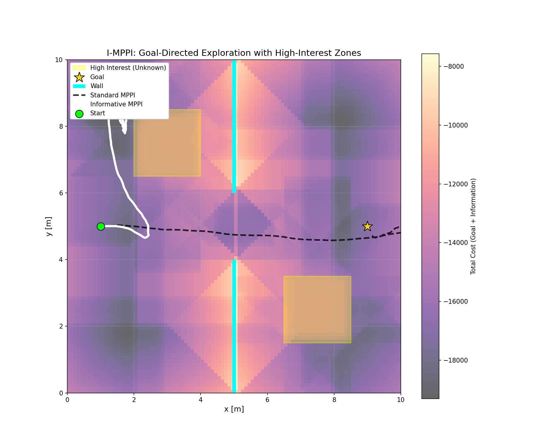
Performance Comparison
The Informative MPPI demonstrates a clear bias towards high-entropy regions of the map. By minimizing the Unified Cost Function, the controller naturally seeks out viewpoints that maximize sensor coverage of unknown space, effectively “falling” into informative gravity wells as predicted by the theory.
Summary: Information as Energy
In I-MPPI, map uncertainty is treated as a High Potential Energy region. The solver naturally seeks to minimize free energy, causing the vehicle to “fall” into informative gravity wells. Calling it Informative MPPI separates the exploration objective from the underlying mathematical solver framework.